3.6 softmax 回归的从零开始实现

1. 初始化模型参数

原始数据集中的每个样本都是 28×28 的图像，输出图像类别有 10 个。本节将展平每个图像，把它们看作长度为 784 的向量。网络只有一层 3.4 softmax 回归#^5f0967，输入的是 784 维，输出 10 维，也就是说：

• 样本矩阵 $X$: 6000×784 的矩阵
• 参数矩阵 $W$ ： 784×10 的矩阵
• 偏置 $b$： 是1×10 的矩阵
• 输出 $Y$: 6000×10 的矩阵

import torch
from IPython import display
from d2l import torch as d2l

batch_size = 256
train_iter, test_iter = d2l.load_data_fashion_mnist(batch_size) # 迭代器的批量大小为256。

num_inputs = 784
num_outputs = 10

W = torch.normal(0, 0.01, size=(num_inputs, num_outputs), requires_grad=True)
b = torch.zeros(num_outputs, requires_grad=True)

2. 定义 softmax 函数

softmax 函数定义如下：

def softmax(X):
    X_exp = torch.exp(X)
    partition = X_exp.sum(1, keepdim=True)
    return X_exp / partition  # 这里应用了广播机制

是对输出 $Y$ 做概率转换，输出 $Y$ 是 6000×10 的矩阵，要沿着横轴方向求和，所以是 axis=1 Pandas 拾遗#^4f157c

3. 定义模型

用 reshape 将每张原始图像展平为向量

def net(X):
    return softmax(torch.matmul(X.reshape((-1, W.shape[0])), W) + b)

4. 损失函数：交叉熵损失

实际标签 y 本身就是一个类别，由交叉熵计算方式，可以用高级索引 Numpy 高级索引（Advanced indexing）#^9d3fd4 在预测矩阵 $Y$ 中选择特定元素：

def cross_entropy(y_hat, y):
	"""输出一行交叉熵损失矩阵"""
    return - torch.log(y_hat[range(len(y_hat)), y])

cross_entropy(y_hat, y)

5. 评估分类精度

def accuracy(y_hat, y):  #@save
    """计算预测正确的数量"""
    if len(y_hat.shape) > 1 and y_hat.shape[1] > 1:
        y_hat = y_hat.argmax(axis=1)
    cmp = y_hat.type(y.dtype) == y
    return float(cmp.type(y.dtype).sum())

accuracy(y_hat, y) / len(y) # 分类准确率

下面定义一个实用程序类 Accumulator，用于对多个变量进行累加。在上面的 evaluate_accuracy 函数中，我们在 Accumulator 实例中创建了2个变量，分别用于存储正确预测的数量和预测的总数量。当我们遍历数据集时，两者都将随着时间的推移而累加。

def evaluate_accuracy(net, data_iter):  #@save
    """计算在指定数据集上模型的精度"""
    if isinstance(net, torch.nn.Module):
        net.eval()  # 将模型设置为评估模式
    metric = Accumulator(2)  # 正确预测数、预测总数
    with torch.no_grad():
        for X, y in data_iter: # 不断叠加计算精度
            metric.add(accuracy(net(X), y), y.numel())
    return metric[0] / metric[1]

class Accumulator:  #@save
    """在n个变量上累加"""
    def __init__(self, n):
        self.data = [0.0] * n

    def add(self, *args):
        self.data = [a + float(b) for a, b in zip(self.data, args)]

    def reset(self):
        self.data = [0.0] * len(self.data)

    def __getitem__(self, idx):
        return self.data[idx]

6. 训练

和线性回归的训练是一样的 3.2 线性回归从零开始实现#^9bc9cb，这里加一些判断更加通用：

6.1 一 个 epoch 的训练

def train_epoch_ch3(net, train_iter, loss, updater):  #@save
    """训练模型一个迭代周期（定义见第3章）"""
    # 将模型设置为训练模式
    if isinstance(net, torch.nn.Module):
        net.train()
    # 训练损失总和、训练准确度总和、样本数
    metric = Accumulator(3)
    for X, y in train_iter:
        # 计算梯度并更新参数
        y_hat = net(X)
        l = loss(y_hat, y)
        if isinstance(updater, torch.optim.Optimizer):
            # 使用PyTorch内置的优化器和损失函数
            updater.zero_grad() # torch 的 SGD 学习器不会除以 batch_size
            l.mean().backward()
            updater.step()
        else:
            # 使用定制的优化器和损失函数
            l.sum().backward()
            updater(X.shape[0]) # 课程内置的 SGD 会除以 batch_size
        metric.add(float(l.sum()), accuracy(y_hat, y), y.numel())
    # 返回训练损失和训练精度
    return metric[0] / metric[2], metric[1] / metric[2]

6.2 动画展示

展示训练函数的实现之前，我们定义一个在动画中绘制数据的实用程序类Animator， 它能够简化本书其余部分的代码。

class Animator:  #@save
    """在动画中绘制数据"""
    def __init__(self, xlabel=None, ylabel=None, legend=None, xlim=None,
                 ylim=None, xscale='linear', yscale='linear',
                 fmts=('-', 'm--', 'g-.', 'r:'), nrows=1, ncols=1,
                 figsize=(3.5, 2.5)):
        # 增量地绘制多条线
        if legend is None:
            legend = []
        d2l.use_svg_display()
        self.fig, self.axes = d2l.plt.subplots(nrows, ncols, figsize=figsize)
        if nrows * ncols == 1:
            self.axes = [self.axes, ]
        # 使用lambda函数捕获参数
        self.config_axes = lambda: d2l.set_axes(
            self.axes[0], xlabel, ylabel, xlim, ylim, xscale, yscale, legend)
        self.X, self.Y, self.fmts = None, None, fmts

    def add(self, x, y):
        # 向图表中添加多个数据点
        if not hasattr(y, "__len__"):
            y = [y]
        n = len(y)
        if not hasattr(x, "__len__"):
            x = [x] * n
        if not self.X:
            self.X = [[] for _ in range(n)]
        if not self.Y:
            self.Y = [[] for _ in range(n)]
        for i, (a, b) in enumerate(zip(x, y)):
            if a is not None and b is not None:
                self.X[i].append(a)
                self.Y[i].append(b)
        self.axes[0].cla()
        for x, y, fmt in zip(self.X, self.Y, self.fmts):
            self.axes[0].plot(x, y, fmt)
        self.config_axes()
        display.display(self.fig)
        display.clear_output(wait=True)

6.3 三次 epoch 的训练

def train_ch3(net, train_iter, test_iter, loss, num_epochs, updater):  #@save
    """训练模型（定义见第3章）"""
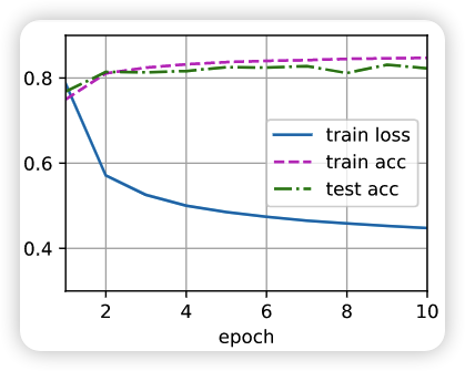
    animator = Animator(xlabel='epoch', xlim=[1, num_epochs], ylim=[0.3, 0.9],
                        legend=['train loss', 'train acc', 'test acc'])
    for epoch in range(num_epochs):
        train_metrics = train_epoch_ch3(net, train_iter, loss, updater)
        test_acc = evaluate_accuracy(net, test_iter)
        animator.add(epoch + 1, train_metrics + (test_acc,))
    train_loss, train_acc = train_metrics
    assert train_loss < 0.5, train_loss
    assert train_acc <= 1 and train_acc > 0.7, train_acc
    assert test_acc <= 1 and test_acc > 0.7, test_acc

• 断言语法见 Python 的 assert（断言）
• 在每个迭代周期结束时，利用 test_iter 访问到的测试数据集对模型进行评估。

lr = 0.1

def updater(batch_size):
    return d2l.sgd([W, b], lr, batch_size)

num_epochs = 10
train_ch3(net, train_iter, test_iter, cross_entropy, num_epochs, updater)

训练结果：

参考文献